# require: matplotlib, seaborn, pytraj
# how? "conda install matplotib seaborn"
import warnings
warnings.filterwarnings('ignore', category=DeprecationWarning)

%matplotlib inline

# add matplotlib and seaborn package
# http://matplotlib.org/
from matplotlib import pyplot as plt

# https://stanford.edu/~mwaskom/software/seaborn/index.html
import seaborn as sns

# use pytraj
import pytraj as pt

# call matrix module
from pytraj import matrix

# load trajectory from file
traj = pt.iterload('tz2.nc', 'tz2.parm7')
traj

pytraj.TrajectoryIterator, 101 frames: 
Size: 0.000503 (GB)
<Topology: 223 atoms, 13 residues, 1 mols, non-PBC>

# caculate rmsd to 1st frame, use only backbone atoms
rmsd_data = pt.rmsd(traj, ref=0, mask='@C,N,O')

# calculate radgyr for all atoms
rg_data = pt.radgyr(traj)
print('rmsd_data', rmsd_data)
print("")
print('rg_data', rg_data)

rmsd_data [  9.60096438e-08   2.40720063e+00   4.12336295e+00 ...,   4.96513980e+00
   5.55340737e+00   4.85867809e+00]

rg_data [  9.4451051    9.57459712  10.19233494 ...,   7.48343543   7.43238185
   7.62039157]

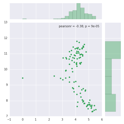
# plot the correlation
# adapted from: 

#sns.jointplot(rmsd_data, rg_data, kind="hex", color="#4CB391")
sns.jointplot(rmsd_data, rg_data, color="#31a354")

#plt.savefig('plot_rmsd_radgyr_correlation.png')

<seaborn.axisgrid.JointGrid at 0x1063d9f28>

Plot rmsd and radgyr correlation¶